We’ve all felt a little lost when we have to analyze product sales data. In this article I’ll show some techniques I like to use when I encounter this type of analysis.

Understand Your Data

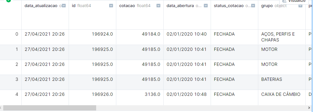
The most important thing for any type of data analysis is understanding the context: what the data represents and what each column or field means. In a perfect hypothetical world, this information will be provided to you by some stakeholder (interested party, or client).

With that in hand, let’s start analyzing our data.

Note: Since the data used is not public — meaning you, dear reader, won’t be able to run the code below — certain details like library imports, auxiliary variable creation, code for chart generation, etc. will be omitted.

1
2
3
4
5
6
7
8

files = [
    '/work/Data/semester_1_2020.csv',
    '/work/Data/semester_2_2020.csv',
    '/work/Data/quarter_1_2021.csv'
]
dataframes = [pd.read_csv(filename, sep=';').dropna(how='all') for filename in files]
df = pd.concat(dataframes, axis=0, ignore_index=True)
df.head()

1

df.info(memory_usage='deep')

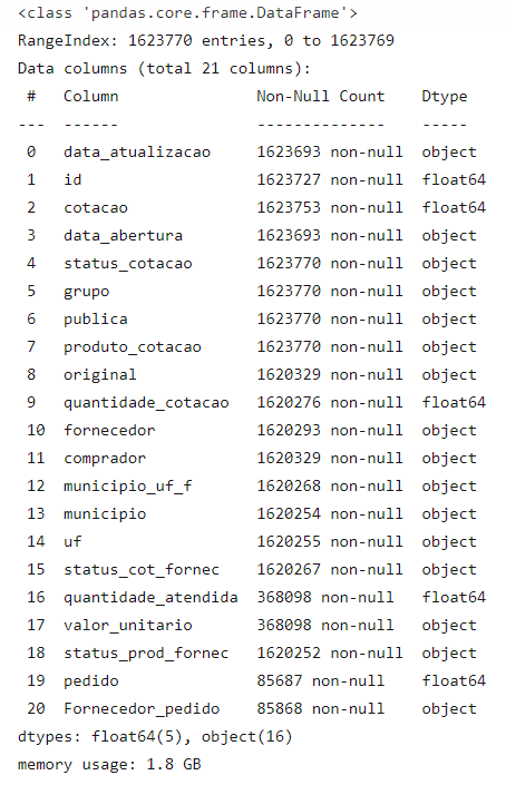
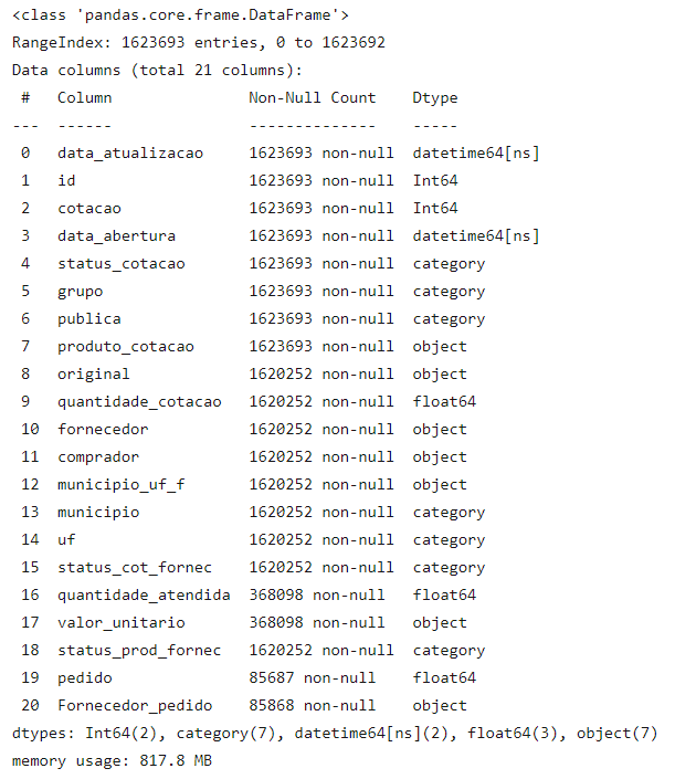
As we can see above, we have some data quality issues. Let’s address them.

The Good Old Data Cleaning

As we can see above, our dataframe is consuming about 1.8 GB of memory, and there are other issues:

• Columns with integers where the content can be null are being treated as float.
• Dates being interpreted as strings.
• Categorical columns being treated as just strings, causing unnecessary memory use.

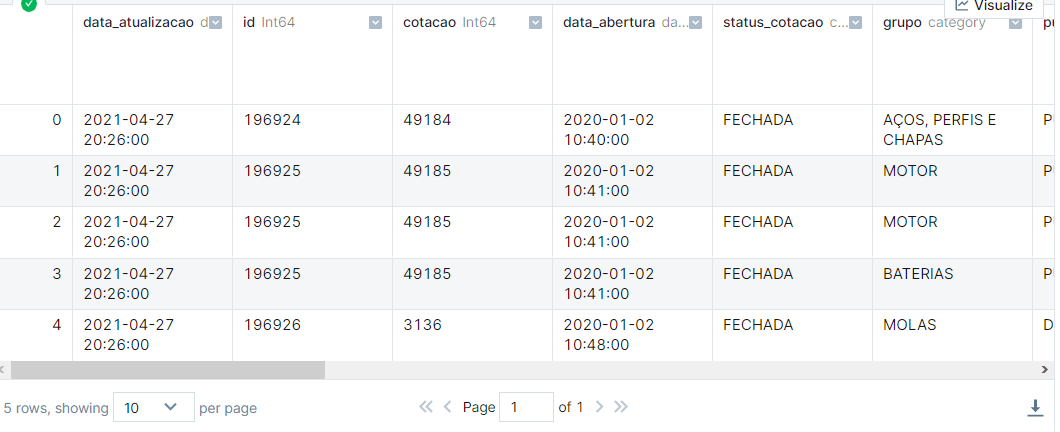
Let’s address these factors.

 1
 2
 3
 4
 5
 6
 7
 8
 9
10
11
12
13
14
15
16
17
18
19
20
21
22

# changing column types to optimize performance and memory
df = df.astype({
    'quote_status':       'category',
    'group':              'category',
    'public':             'category',
    'city':               'category',
    'state':              'category',
    'supplier_status':    'category',
    'product_status':     'category',
    'id':                 'Int64',
    'quote':              'Int64',
})
# converting date columns
df['updated_at'] = pd.to_datetime(df['updated_at'], format='%d/%m/%Y %H:%M')
df['opened_at']  = pd.to_datetime(df['opened_at'], format='%d/%m/%Y %H:%M')
# removing invalid/empty rows
df = df[df['id'].notna()]
df = df[df['opened_at'].notna()]
# sorting by opened_at
df.sort_values('opened_at', inplace=True)
df.reset_index(inplace=True, drop=True)
df.head()

1

df.info(memory_usage='deep')

With the changes, in addition to the significant performance improvement we’ll see, we also saved about 1 GB of memory.

Now let’s actually analyze our data.

Product Groups

In our dataset we have a column called “group” that indicates which category a product belongs to. Based on it we’ll generate some charts to understand buying behavior in our dataset.

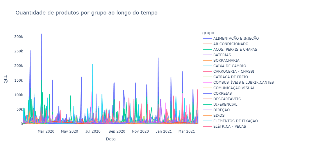
Beautiful, isn’t it? Of course not! However, even with a so-called “ugly” chart we can draw a number of insights:

• First: we don’t have a daily sales frequency for the vast majority of groups. We can see this thanks to the visible sales spikes that in some groups occur monthly.
• Second, despite having dozens of different groups, some groups appear to have a higher quantity of sales than others.
• Third, the “air conditioning” group appears to have visible seasonal sales throughout the year, probably due to climate factors (seasons of the year).

Below we can see a chart with the 10 best-selling product groups.

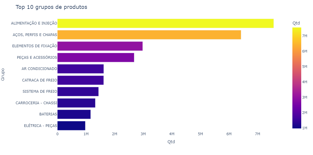
The “food and injection” and “steels, profiles and sheets” groups hold most of the sales quantity (in the top 10).

Let’s now look at a correlation Heatmap between these product groups.

1
2
3
4
5
6
7
8

# creating time series with product groups and quoted quantity
df_products_group_ts = df[['group', 'opened_at', 'quote_quantity']].copy()
df_products_group_ts['opened_at'] = df_products_group_ts['opened_at'].dt.date
df_products_group_ts = df_products_group_ts.groupby(['opened_at', 'group'])[['quote_quantity']].sum().reset_index().dropna()
df_products_group_ts.set_index('opened_at', inplace=True, drop=False)
df_products_group_ts.sort_index()
df_products_group_ts = df_products_group_ts[df_products_group_ts['quote_quantity'] > 0]
df_products_group_ts.head()

 1
 2
 3
 4
 5
 6
 7
 8
 9
10
11
12
13
14
15
16
17
18
19
20
21
22
23
24

# generating correlation matrix
df_products_group_corr = df_products_group_ts.pivot('opened_at', 'group', 'quote_quantity').fillna(0).corr()
df_products_group_corr = df_products_group_corr * 100
mask = np.triu(np.ones_like(df_products_group_corr, dtype=bool))
rLT = df_products_group_corr.mask(mask)
fig = go.Figure(
    data=go.Heatmap(
            z=rLT.values,
            x=rLT.columns,
            y=rLT.index,
            colorscale='hot_r',
            name=''
    )
)
fig.update_layout(
    title='Product Correlation Heatmap',
    width=1500,
    height=1500,
    yaxis_autorange='reversed',
    paper_bgcolor='rgba(0,0,0,0)',
    plot_bgcolor='rgba(0,0,0,0)'
)
fig.update_traces(hovertemplate='%{x}<br>----<br>%{y}<br>=%{z:.2f}%')
fig.show()

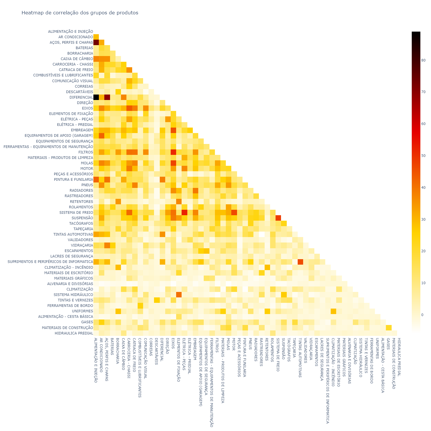
A correlation heatmap is a table showing correlation coefficients between variables. Each cell in the heatmap shows the correlation between two variables.

In statistics it is represented by the letter r.

Correlation is a number that varies between -1 and 1 (in our case this number was transformed to values between -100 and 100).

Below is a chart with the 5 highest correlations.

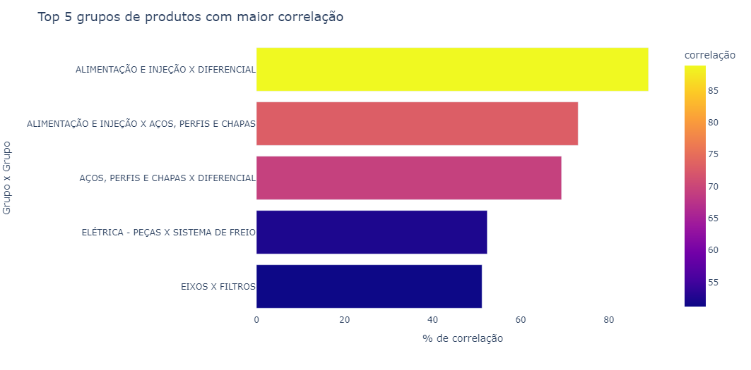
A correlation heatmap is one of my favorite types of charts. From it we can see correlations — in this case of sales — that sometimes may not be so obvious, for example, the correlation between “electrical - parts” and “brake system”.

Purchase Behavior vs. Weather Data

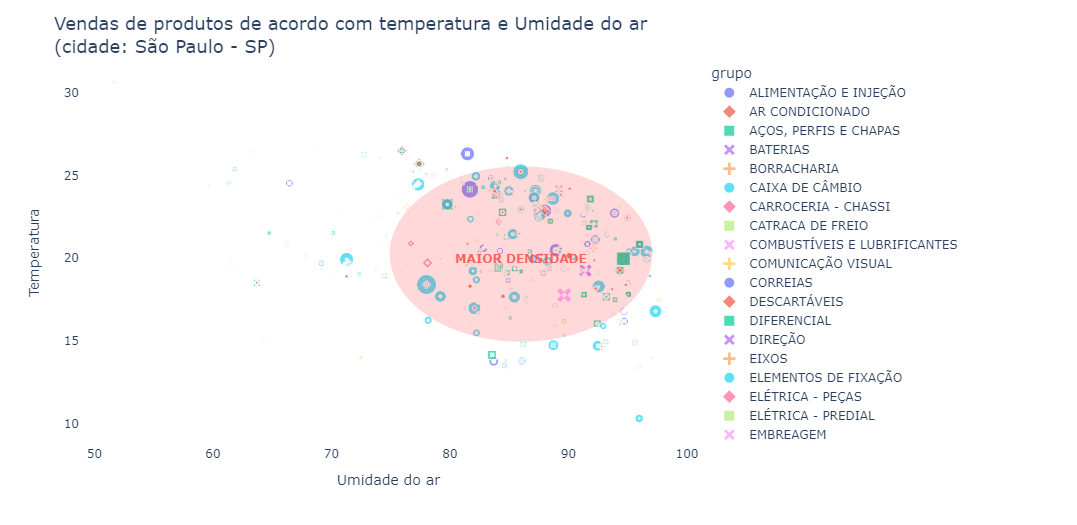
Since we raised the hypothesis that some product groups might have some correlation with climate situations, let’s cross-reference this information.

Temperature and humidity data for the city of São Paulo were crossed with purchases made on that day. Temperature data was extracted from the National Meteorology Institute website.

Predicting Purchase Behavior

Based on the previous analyses, sales for the “air conditioning” group appear to have some seasonality. Let’s try to create a model to predict sales for this product group in the coming months.

 1
 2
 3
 4
 5
 6
 7
 8
 9
10
11
12
13

date_end = datetime.date(2021, 1, 1)
df_air_conditioning_group_SP_ts = (
    df_products_group_SP_ts
    .query('group == "AIR CONDITIONING"')
    .rename(columns={'opened_at': 'ds'})
)
# smoothing data by applying 7-day moving average
df_air_conditioning_group_SP_ts['y'] = df_air_conditioning_group_SP_ts['quote_quantity'].rolling(7).mean()
# using facebook prophet to forecast the time series
prophet_model = Prophet(
    yearly_seasonality=True,
    daily_seasonality=True,
).fit(df_air_conditioning_group_SP_ts.query('ds<@date_end'))

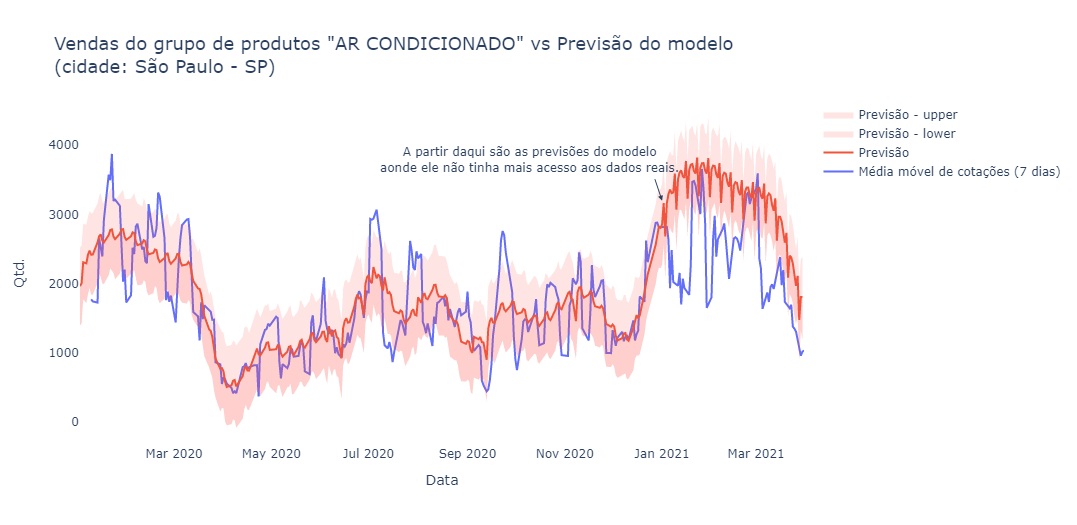
Incredible — despite not being perfect, the model apparently managed to correctly identify and predict the seasonality of the data.

Below are some seasonalities and trends identified by the model.

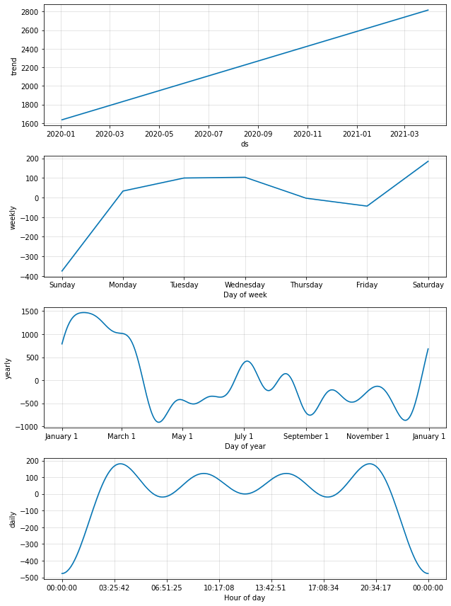
Based on the charts above we can draw some very interesting insights:

• Most purchases occur during business days between 3:30 AM and 8:30 PM.
• Sales tend to drop a bit on Thursdays and Fridays, and due to this accumulation the highest sales peak occurs on Saturdays.
• The day of the week with fewest sales is Sunday.

Market Basket Analysis

First, what is it? Market basket analysis is a technique whose objective is to predict customers’ purchasing decisions — that is, when the customer buys product X they also tend to buy product Y together.

This is an indispensable type of analysis when analyzing sales data, so let’s implement it.

1
2
3
4
5
6
7

df_basket = df.groupby(['quote', 'product'])['quote_quantity'].sum().unstack().reset_index().fillna(0).set_index('quote')
df_basket = df_basket.applymap(lambda item: 0 if item <= 0 else 1)
df_fpgrowth = fpgrowth(df_basket, min_support=0.04, use_colnames=True, max_len=2)
df_fpgrowth = df_fpgrowth[df_fpgrowth['itemsets'].map(len) > 1]
df_fpgrowth['itemsets'] = df_fpgrowth['itemsets'].map(list)
df_fpgrowth.sort_values('support', ascending=False, inplace=True)
df_fpgrowth.reset_index(inplace=True, drop=True)

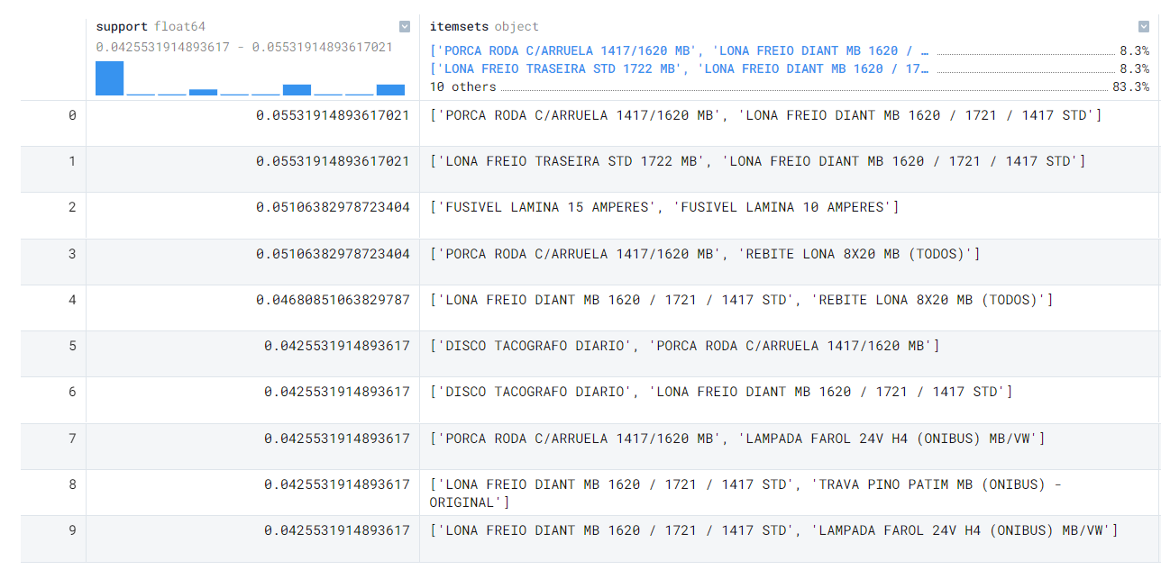
Support is calculated as follows:

1

support = transactions_where_items_appear / total_transactions

Just like the heatmap analysis, the market basket analysis provides a sensational view of the sales correlations in our data.

Conclusion

Please tell me your opinion below!

What did you think of the analysis? Would you have done something more or different?